Sensible. One of the more common words we see these days in regards to player movements. Fans and analysts ask “Is the deal sensible?” in line with questions of the transfer fee and stylistic fit of the player into a team’s tactical approach. We often see comparisons of who “might have been bought” for the fee as alternatives, or a number of data points in playing performances used to justify or criticize the acquisition for the club.
There is another perspective to consider, however, and that is the perspective of business. Professional sport is a business and spending on assets must be justified. How do we justify the wages a club spends on the player? That is what we will look to explore in this article.
Looking to Baseball
When it comes to performance data, all sports look to baseball. Baseball is a sport that is incredibly easy to quantify, which gives us a wealth of data at any given time. One of the more valuable [some could argue most valuable] metrics that baseball has given us is Wins Above Replacement, or WAR. WAR is officially defined by Major League Baseball as a measurement of “a player’s value in all facets of the game by deciphering how many more wins he’s worth than a replacement-level player at his same position (e.g., a Minor League replacement or a readily available fill-in free agent).” Wins Above Replacement is a metric that has tried to be replicated [and in some cases, successfully implemented] across almost all sports, but it is fair to say the translated metrics do not have the same impact that WAR has on baseball due to how baseball is played.
To paint a clearer picture of WAR and the value it brings, I’ve collected data on 764 Major League Baseball players from the website FanGraphs. In the visuals below, we will see each player’s WAR for the 2022 MLB Regular Season and their base salary for the 2022 season.
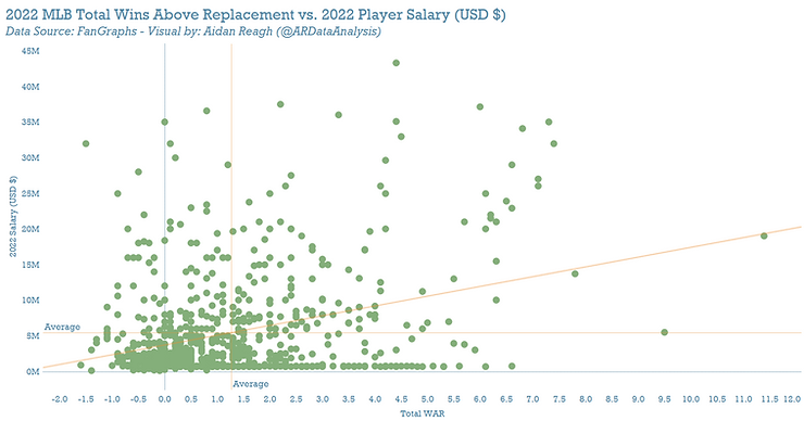
In this first visual, we see WAR with each player’s yearly base salary. We obviously see the main cluster of players on the lower value contracts, with many of them around the average or performances of 0.0. A key takeaway here to notice is the general trend. The better the WAR, the more the player costs a team. This shows that Major League Baseball [which has become arguably the smartest operating of sports leagues thanks to the wealth of data at key decision makers’ fingertips] tends to correctly spend their money. You do, however, see a handful of the most expensive players are actually below average in their WAR. Now that we’ve seen this, let’s take a look at it from a different perspective.
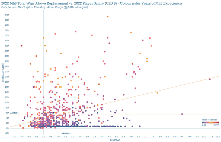
If we take the same variables and look at the years the player has been playing in Major League Baseball, we see it pays to be a veteran. This is where we will transition back to football as a focus. Younger players are often assets that can come at a lower price than players that are in their prime or on their “last big contract”. It pays to be experienced in sport.
In the next sections of this post, all data will be in reference to the 2021-22 German Bundesliga season. I’ve selected the German Bundesliga due to the accessibility of public data on the league as well as the relatively balanced wage distribution across the league, making it a bit more straightforward to use as an example. Wage data has been obtained from Capology/Football Reference. This data is not perfect, but suitable enough for a hypothetical study exploring different models of asset evaluation. If you are interested in learning more or have questions about Capology’s data, please click here. Now it is time to ask “how can we evaluate our assets?”
Evaluating Our Assets
A quick way to evaluate our assets is simply asking “How often are they on the pitch? Are we paying for an expectation of regular minutes from someone who isn’t good enough to earn regular minutes?” Another way to evaluate if the assets are justifying their cost is to compare their cost to their productivity. If I may reference a primary influence of mine in 21st Club [Volumes 1 and 3 of Changing the Conversation], there are a couple of ways to create an ideal wage model.
Model A: Squad Role
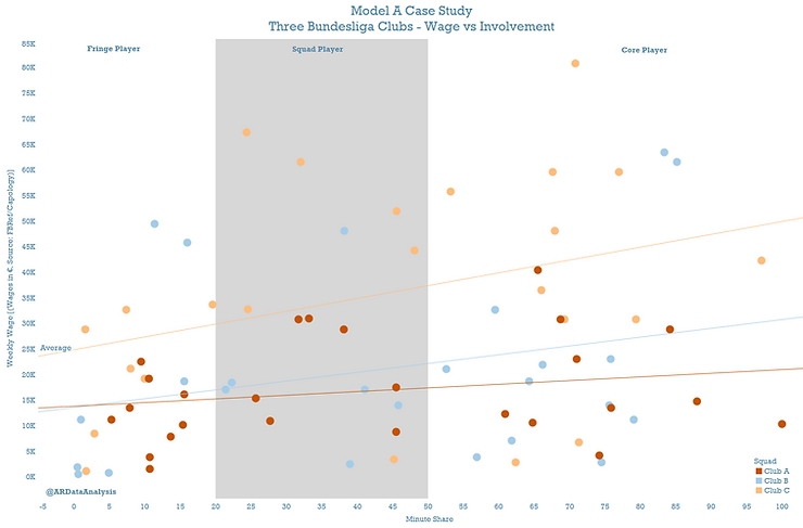
The Squad Role model takes the concept that you have three categories of player involvement. These three categories are defined by minute involvement. The Squad Role Model suggests your wage bill should follow this framework:
- Core Player: The Core Player should be involved in at least 50% of all minutes available (ideally as close to 100% as possible) and should be paid in line with this, falling in the category of the upper third in terms of the wage bill.
- Squad Player: The Squad Player should be involved between 20% and 50% of all minutes available and should be paid in the middle third bracket of the wage bill.
- Fringe Player: The Fringe Player should only be involved in less than 20% of all minutes available [think youth, legacy players, or depth goalkeepers] and should make up the lower third bracket of the wage bill.
Model B: Player Ranking
The Player Ranking model takes the 25-man squad and groups the players in relative ability compared to the squad. Once this grouping is completed, it is recommended that an optimal wage bill is distributed to the players as follows:
- The top 5 players receive 40% of the total wage bill
- Players ranked 6 – 10 receive 25% of the total wage bill
- Players ranked 11 – 15 receive 15% of the total wage bill
- Players ranked 16 – 20 receive 12% of the total wage bill
- Players ranked 21 – 25 receive 8% of the total wage bill.
Models A and B are both proposed by 21st Group, but now I’d like to fall back to our baseball influences and suggest the application of data for Model C, a less subjective Model B:
Model C: The Data Model
While Football does not yet have a reliable WAR metric, there are a number of metrics being identified by clubs as “critical to player evaluation”. Any of these metrics, indexes, scores, etc. can be used here, but for the sake of what we have available to use in a hypothetical post, I will be using InStat’s Index tool. You can find out more in detail about InStat’s Index here, but a quick overview is this is an algorithm that considers the player’s contribution to success and establishes a player’s relative ability.
When calculating how much a player is worth, this model simply aims to show players who score higher in your metrics should be valued more, and that should be reflected in the player’s wages.
Testing the Models
Before we apply the 2021-22 Bundesliga to each of these models, we must know that any ideal asset evaluation should look like this [see below] – the more we value the asset, the more we should be spending on it.
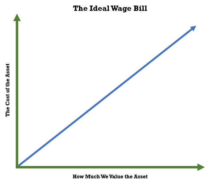
Now that we have our ideal wage bill visualized, we can apply Model A. With 11 players and 34 games of 90 minutes available to the Bundesliga, there are 33,660 total team minutes available, or 3,060 per player to define our minute share.
For our application of Model A, I’ve selected three Bundesliga clubs with relatively similar wage bills [see below] to see who is closest to Model A’s ideals. As it turns out, Club C follows it closest, with the general trend being the more a player costs, the more involved he is. Club B and C are not really fitting into Model A, so if we were to judge a team purely on this [please know, we shouldn’t, we must always remember context], we could say that Clubs B and C are not handling their wage bill efficiently. That they are spending more than they should for players who are not involved in the capacity that they should be.
We will come back to Model B later with a specific team, but first, I want to look at Model C. Remember the ideal result for Model C is a player with a higher index score is paid more. With this model being visualized for the full league rather than just a club, this gives us a chance to identify high performers who might not be getting paid their true worth, similar to our MLB visuals that utilized WAR. Note: Due to Bayern Munich’s wage bill operating completely differently from the rest of the league [Bayern paying €2.85m more than the league’s second-highest wage bill, Dortmund], they have been removed from this visual to make the visual a bit easier to read and identify assets being undervalued compared to the rest of the league. All players will be marked with blue or green. If a player has moved clubs [excluding loans] in the Summer 2022 Movement Window, they will be identified with a green point.
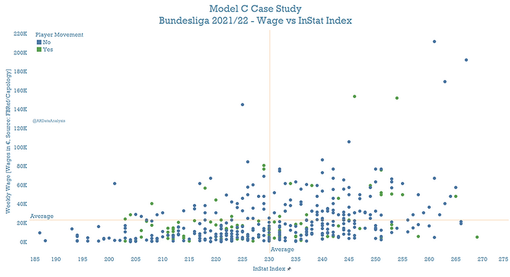
Our first impression should be immediately that this is a bit cramped, so before we start any analysis let’s compress our Model C visual and bring the weekly wage maximum to 100k. This essentially removes a few key players from Borussia Dortmund as well as Andre Silva of RB Leipzig.
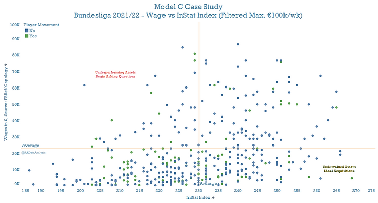
Now that the visual is a bit easier to process and the wages are in a filter that is more accessible for the average Bundesliga club, we can begin analyzing. In quadrant II (upper left) we should be noting players at our club and asking “What do they bring to the club? Is it replaceable?” – If you answer “Yes” to the second question, then this is an ideal asset to move on from. As we can see, some clubs decided it was smart to sell, as 20% of players in this category moved on this past summer.
Looking to quadrant IV (bottom right) we should be noting players at other clubs as potentially undervalued assets that we can potentially acquire, or we can identify the players at our own club as ideal candidates for a contract extension to reward their positive performances. Of the 115 players in this category, 21% of players saw summer moves come their way.
With Model C, any scoring system/key performance indicator can be used against wages as a potential asset evaluation method, but remember to consider qualitative assets that might not be visible in quantitative metrics when considering a final evaluation.
Coming back to Model B, rather than me ranking the 25 players in a subjective way, we will be integrating the InStat index to create the ranking. For Model B, our example club will be Eintracht Frankfurt. Player Wages are back to being sorted by % of their club’s total wage, similar to Model A.
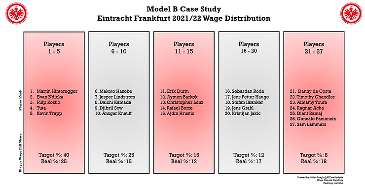
What we can see here is Frankfurt finds itself one tier ahead of the target until we get to players 16 and on. These players create a higher actual % than the ideal target and could be considered deadweight players, or fringe players who might not meet the standards of our asset evaluation. Note: Real % falls short of 100 due to player movements before the end of the season that contributed to a wage bill but an InStat Index score for ranking was unavailable.
Every model has pros and cons to it and can be used to answer different questions. All of these models can also be changed in method to fit the exact club model of asset evaluation. With the three models discussed, which do you prefer? Do you feel one comes closer to fitting “the ideal wage bill”?
Final Notes
As we end this article, one thing must always be remembered: Football is not Moneyball – it is far too unpredictable. We can find ways to show if our assets [aka our players] meet what we deem acceptable performances compared to what we are paying. Still, we must never forget the context of the game and take it into consideration. Players are humans, not robots. For example, a leader will always bring additional value to what the changing room gains with his/her presence. Always ask “why” before you make a decision.
Data in this article is sourced from FanGraphs (MLB Data), Football Reference and Capology (Player wages), and InStat (InStat Index). Many ideas/concepts here, including theories on wage optimization, come from the brilliant work of 21st Club. If you are interested in seeing more visuals, articles, or discussions similar to this, you can find me on Twitter @ARDataAnalysis. On a personal note, much of my writing would not happen if not for my partner, Lacy. Be it helping me solve whatever data issue I have or simply being an amazing part of my life every day, I cannot thank her enough for all she does every day.
By Aidan Reagh

